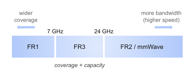
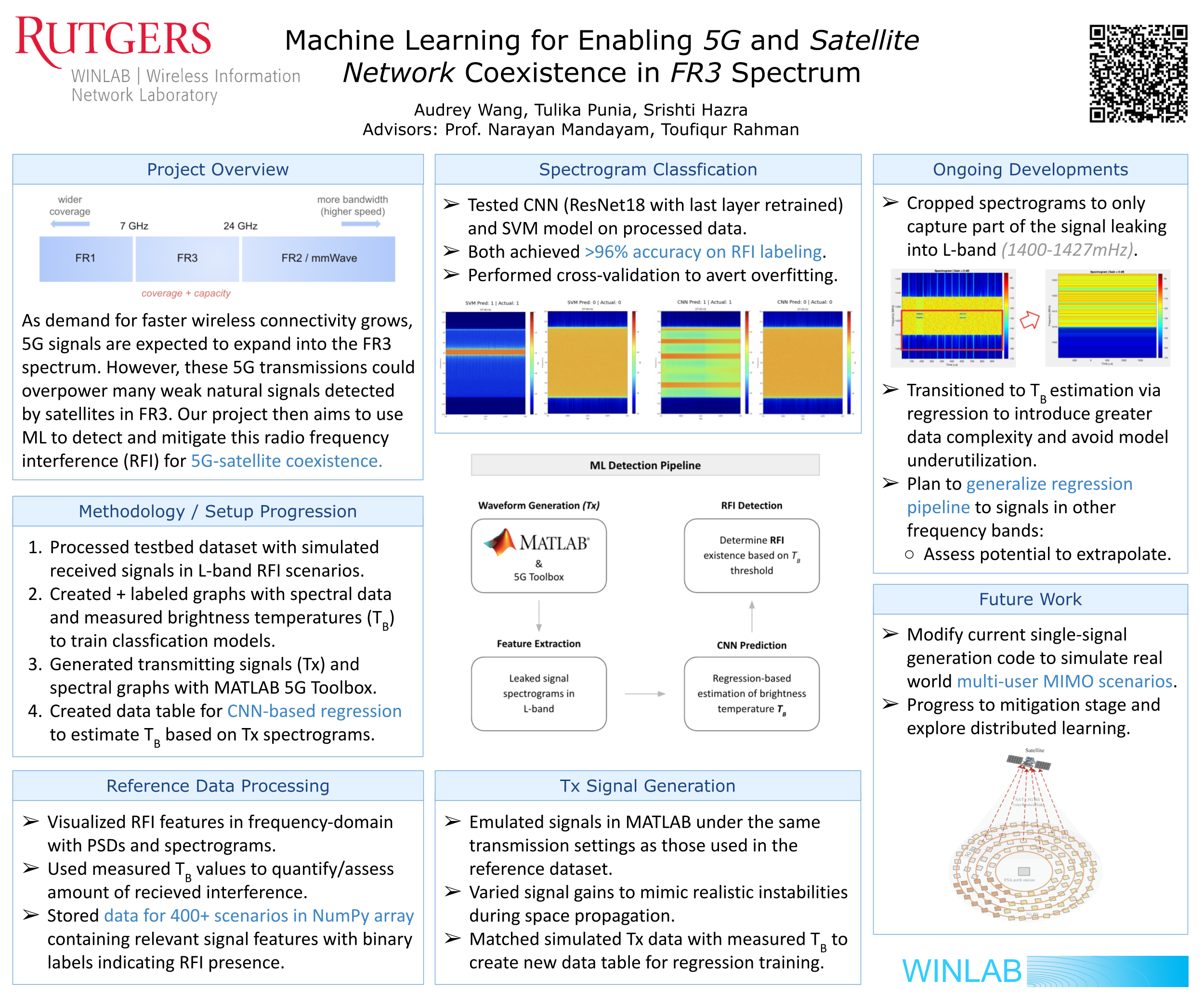
Machine Learning for Enabling 5G and Satellite Network Coexistence in FR3 Spectrum

WINLAB Summer Internship 2025

Group Members: Audrey Wang, Tulika Punia, Srishti Hazra

Week 1 (5/27 - 5/29):

Slides: ​Week 1 Presentation

Progress:

• Conducted literature review on relevant research papers
  1. ​Modeling the Impact of 5G Leakage on Weather Prediction
  2. ​Will Emerging Millimeter-Wave Cellular Networks Cause Harmful Interference to Weather Satellites?
  3. ​How Does the Growth of 5G mmWave Deployment Affect the Accuracy of Numerical Weather Forecasting?
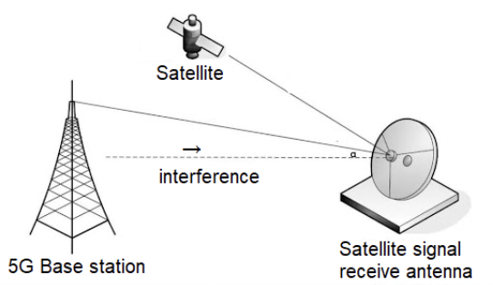
• Understood the high level idea of what Radio Frequency Interference(RFI) and frequency allocations are
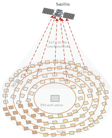
• Explored how ML can be implemented to minimize the interference between satellite and 5G in different spectrums

Week 2 (6/2 - 6/5):

Slides: ​Week 2 Presentation

Progress:

• Familiar with the pros and cons of the different approaches to beam-forming, especially the benefits of ML application
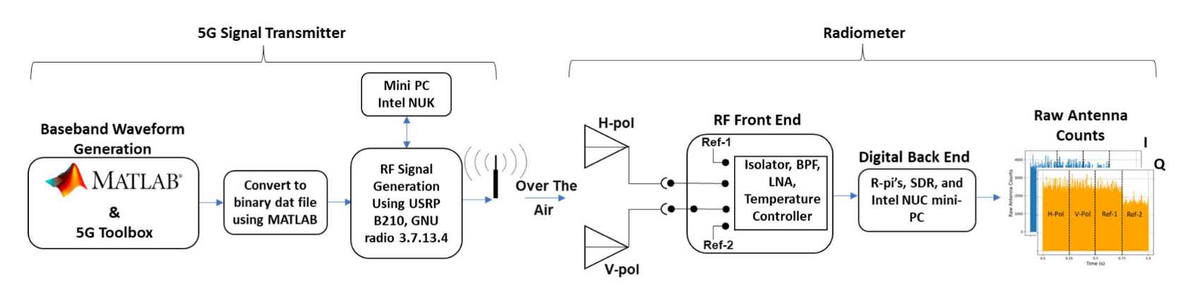
• Read research papers related to a physical-testbed-generated RFI dataset, and got familiar with the data generation process:
  1. ​A Physical Testbed and Open Dataset for Passive Sensing and Wireless Communication Spectrum Coexistence
  2. ​Microwave Radiometer Calibration Using Deep Learning With Reduced Reference Information and 2-D Spectral Features
  3. ​Radio Frequency Interference Detection for SMAP Radiometer Using Convolutional Neural Networks

Week 3 (6/9 - 6/12):

Slides: ​Week 3 Presentation

Progress:

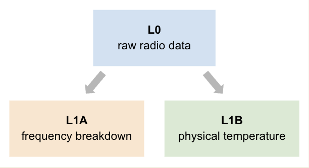
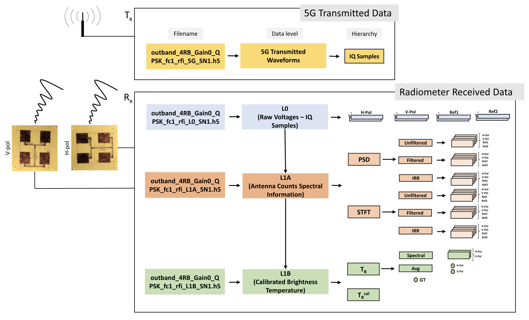
• Grasped the comprehensive testbed pipeline and understood how calibrated higher-level data were obtained from raw I/Q signals
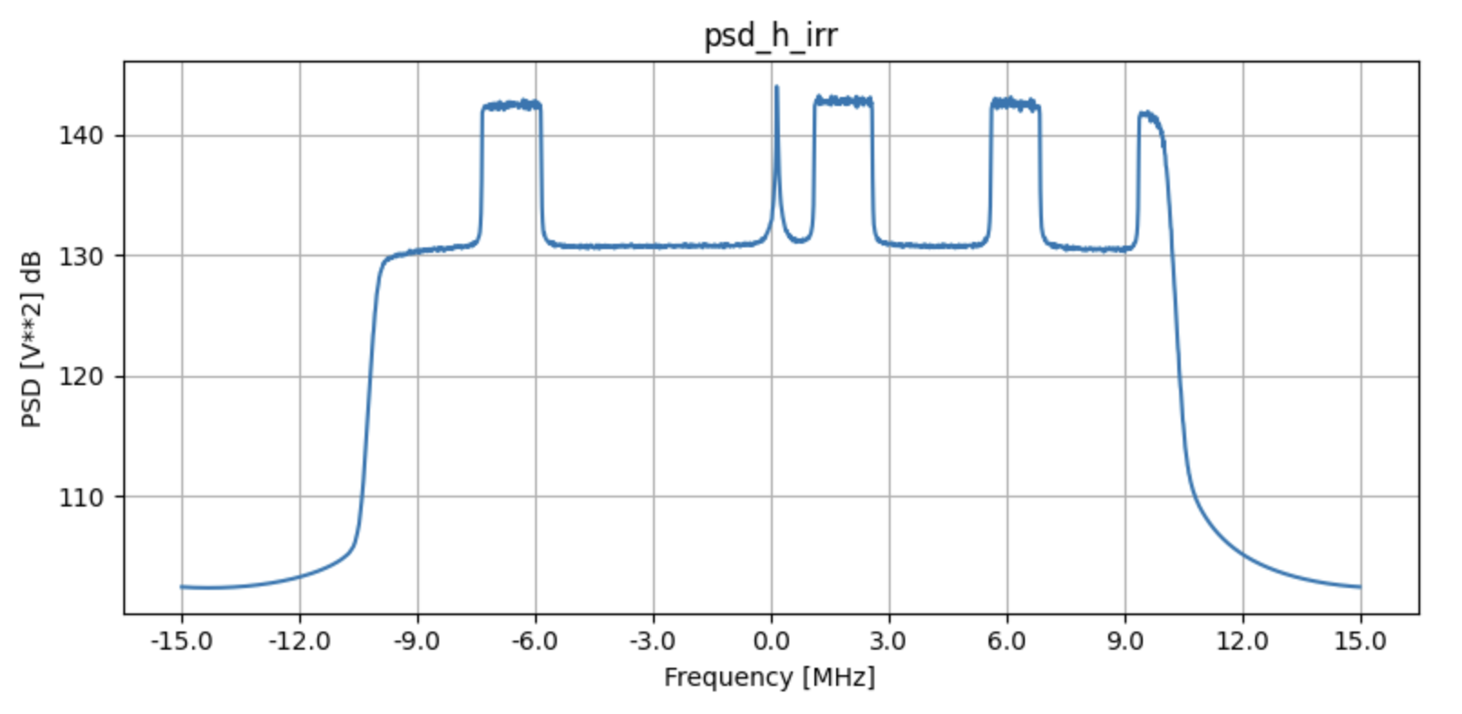
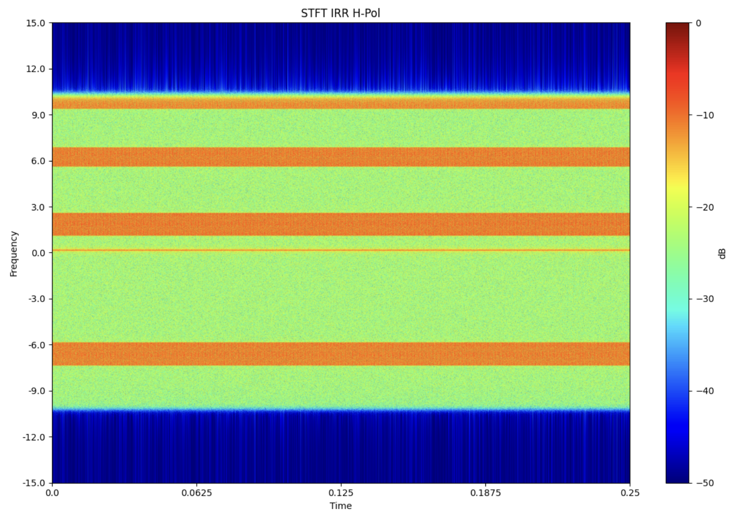
• Began to process data with Numpy and h5py, generating Power Spectral Density(PSD) graphs and spectrograms from L1A data
• Utilized the radiometer's ability to interpret all received power as thermal radiation to quantify RFI by detecting abnormal temperature increases
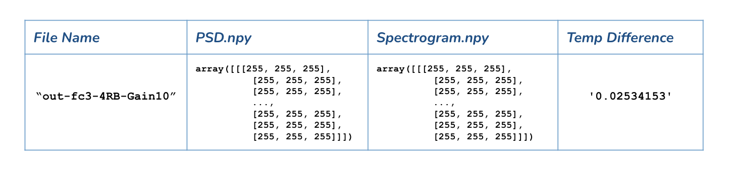
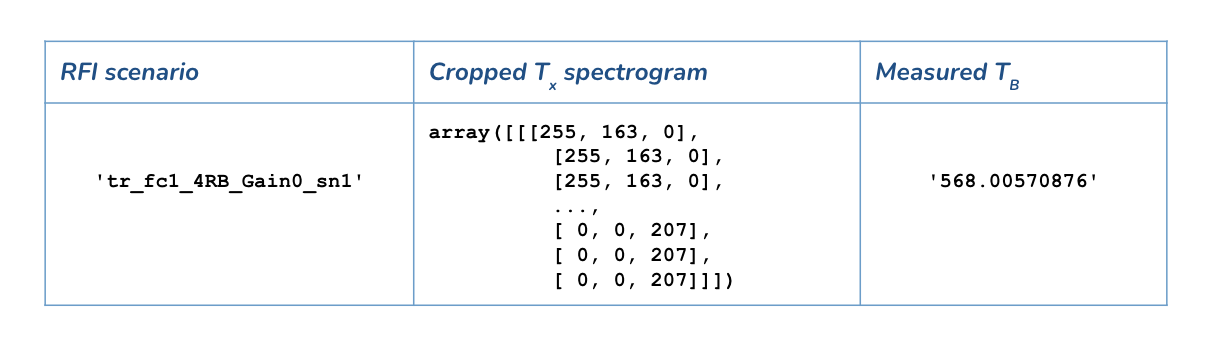
• Saved plotted graphs into a 2D Numpy array for future model training use (4 columns: RFI Scenario | PSD | Spectrogram | Temp Difference)

Week 4 (6/16 - 6/19):

Slides: ​Week 4 Presentation

Progress:

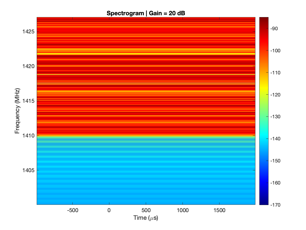
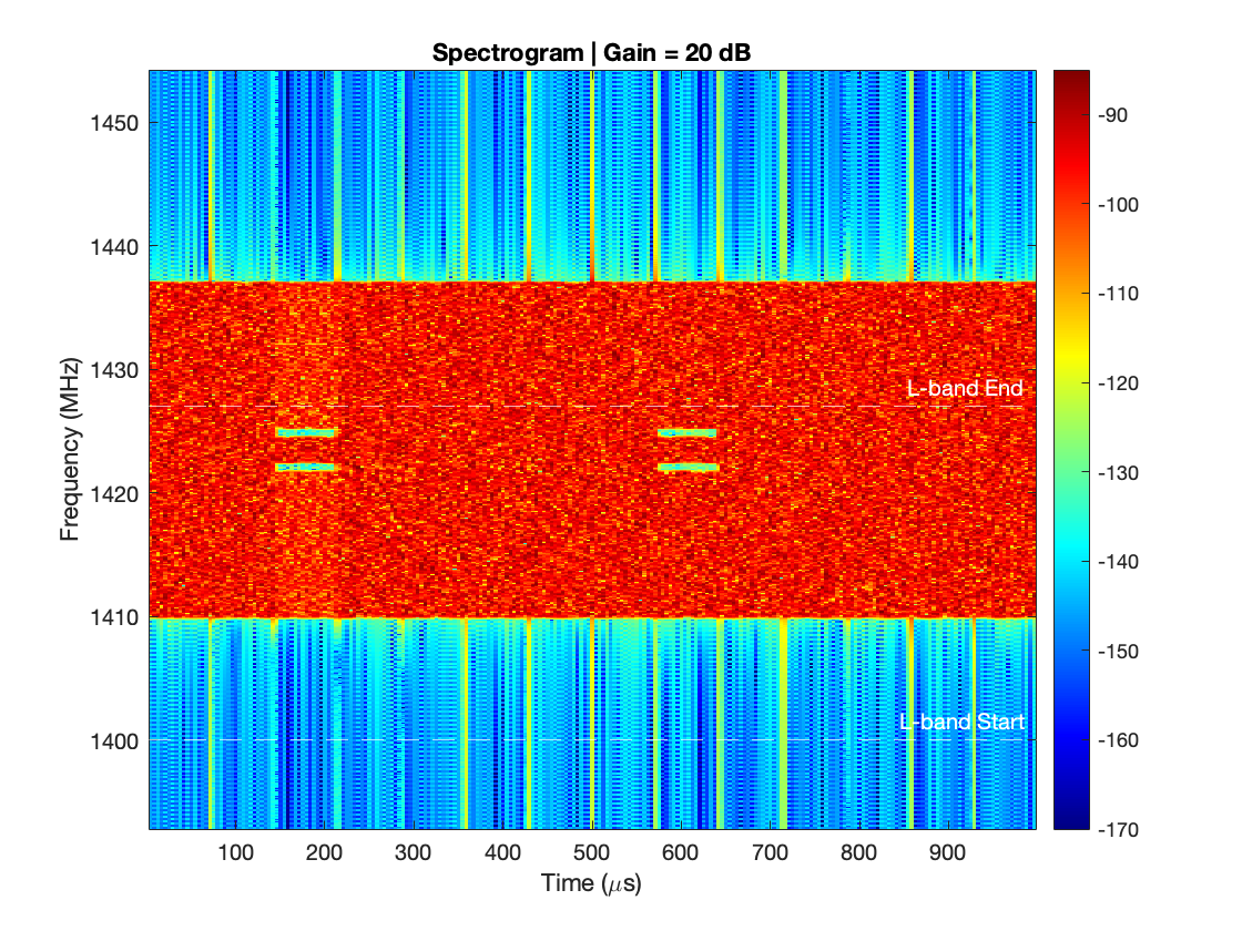
• Continued generating PSDs and spectrograms using Jupyter Notebook (link to ​code)

• Sample PSD and spectrogram for RFI scenario "tr_fc0_4RB_Gain-20_sn2" (transition band; central frequency 0; 4 resource blocks; gain -20; sample number 2)

Week 5 (6/23 - 6/26):

Slides: ​Week 5 Presentation

• In progress to generate all graphs for fc1, 2, 3 for both a) transition-band and b) out-of-band scenarios

• Code used for generating spectrograms and converting into Numpy arrays to facilitate easier data processing in the future:

  def plot_spect(dataset, title,min_value,max_value,normalized=False, save=None):
      if normalized:
          global_maximum = np.amax(np.abs(dataset))
      else:
          global_maximum = 1
  
      #normalize received power and convert into dB scale)
      y_res = 20 * np.log10(np.abs(dataset) / global_maximum) 
  
      fig = plt.figure(figsize=(12, 8))
      im = plt.imshow(y_res, origin='lower', cmap='jet', aspect='auto', vmax=max_value, vmin=min_value)
      plt.colorbar(label='dB')
  
      yaxis = np.ceil(np.linspace(-15, 15, 11))
      ylabel = np.linspace(0, len(y_res), 11)
      xaxis = np.linspace(0, .25, 5)
      xlabel = np.linspace(0, len(y_res[1]), 5)
  
      plt.title(title)
      plt.yticks(ylabel, yaxis)
      plt.xticks(xlabel, xaxis)
      plt.xlabel('Time')
      plt.ylabel('Frequency')
      plt.tight_layout()
  
      #save the RGB values of the plot as a Numpy array
      fig.canvas.draw()
      img_rgba = np.frombuffer(fig.canvas.tostring_argb(), dtype=np.uint8)
      img_rgba = img_rgba.reshape(fig.canvas.get_width_height()[::-1] + (4,))
      img_rgb = img_rgba[:, :, [1, 2, 3]]
  
      return img_rgb
  

Week 6 (6/30 - 7/3):

Slides: ​Week 6 Presentation

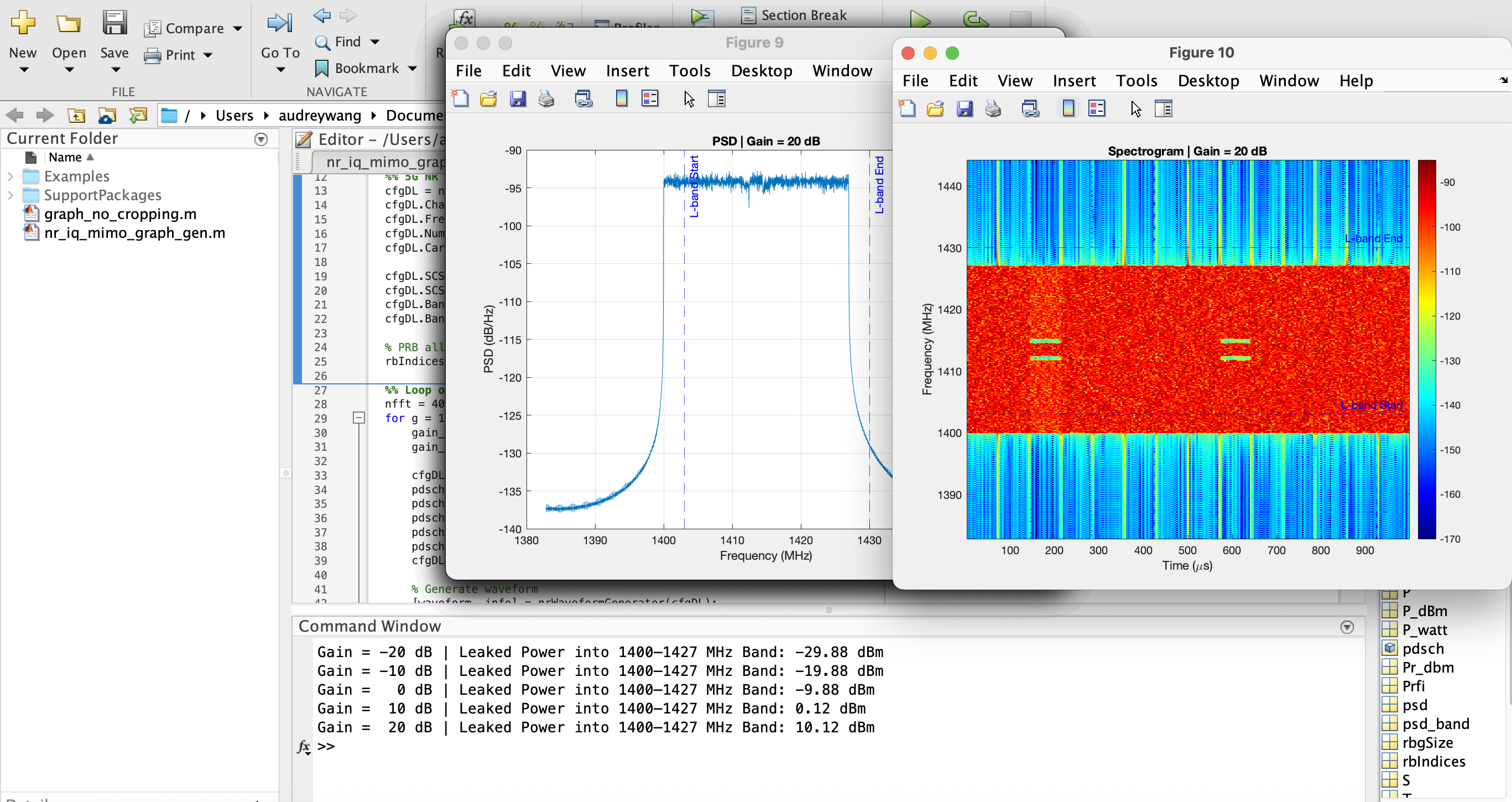
• Finished generating 348 sets of graphical data for the following inference scenarios:
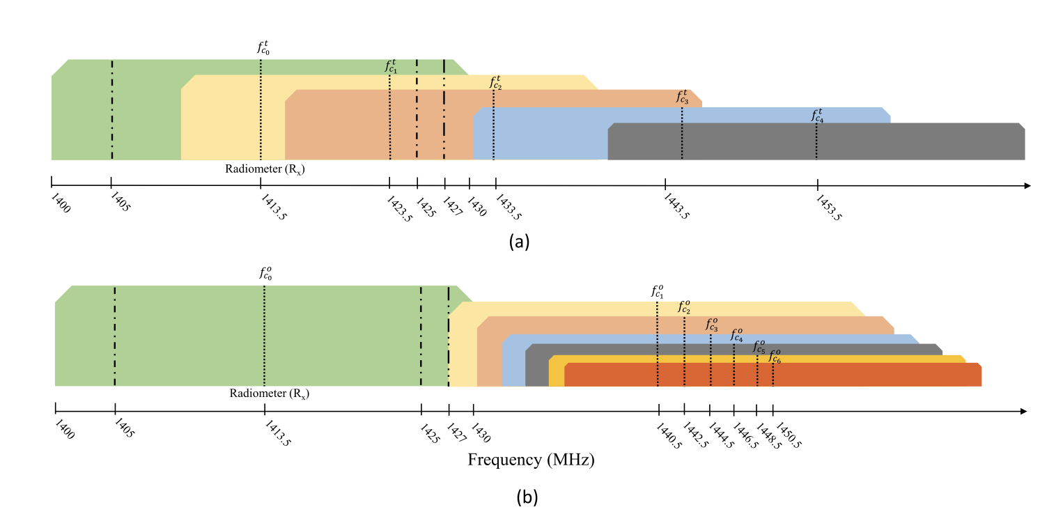
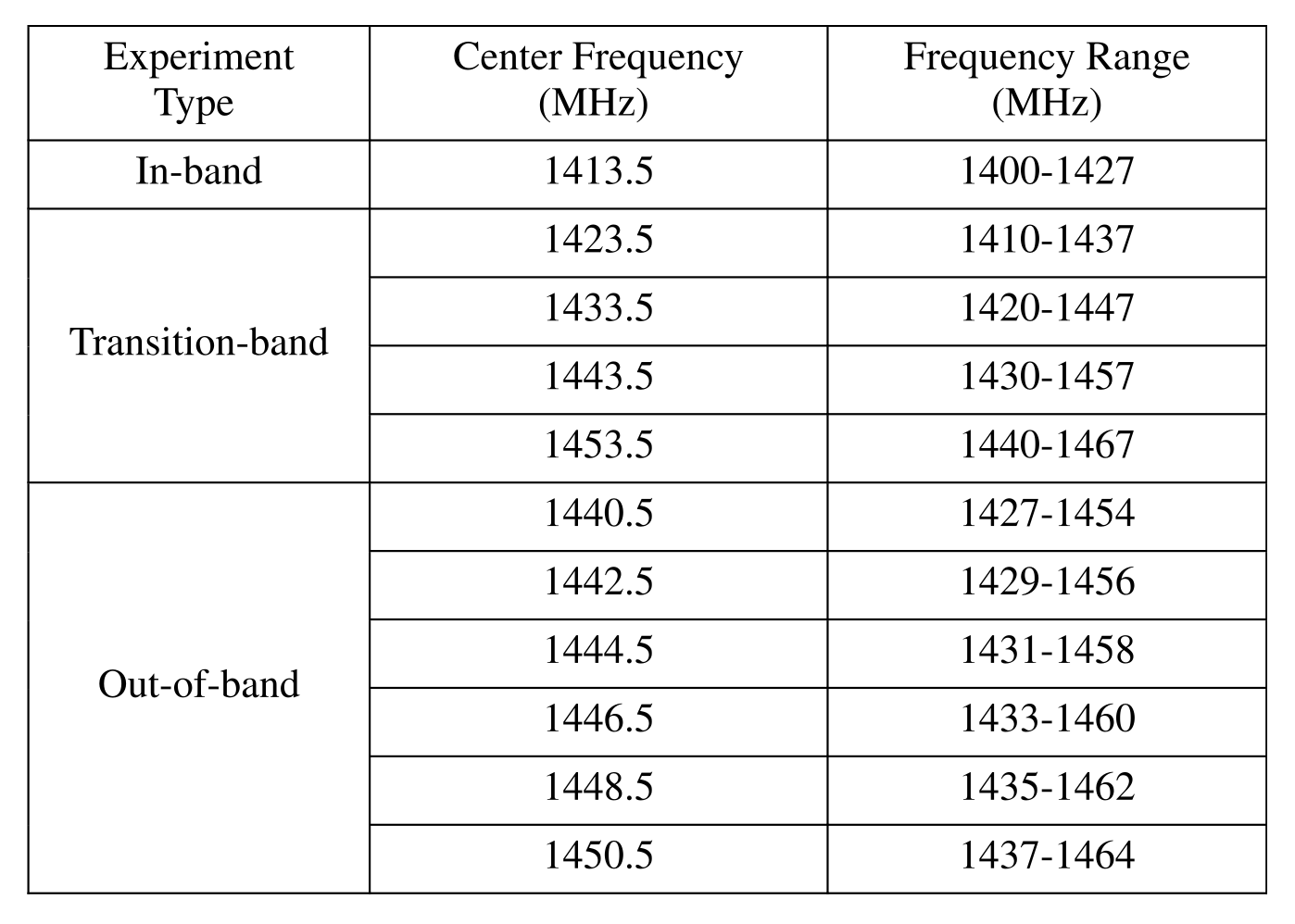
  1. Center frequencies 1423.5mHz(fc1), 1433.5mHz(fc2), 1443.5mHz(fc3) for transition band
  2. Center frequencies 1440.5mHz(fc1), 1442.5mHz(fc2), 1444.5mHz(fc3) for out-of-band

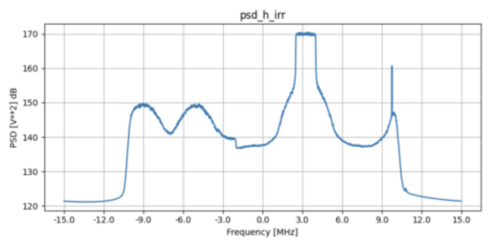
• Identified clean vs. RFI-contaminated signal shapes in Power Spectral Density (PSD) plots:
  1. Uniform (Clean, L): flat-top spectrum, power emitted uniformly across entire bandwidth
  2. Spikes (RFI, R): abrupt, sharp spikes in power at random frequencies

• Determined brightness temperature thresholds for various gain levels and labeled the dataset as clean = 0 or RFI-contaminated = 1
  • Link to ​code

Week 7 (7/7 - 7/10):

Slides: ​Week 7 Presentation

Progress:

• Machine learning models:
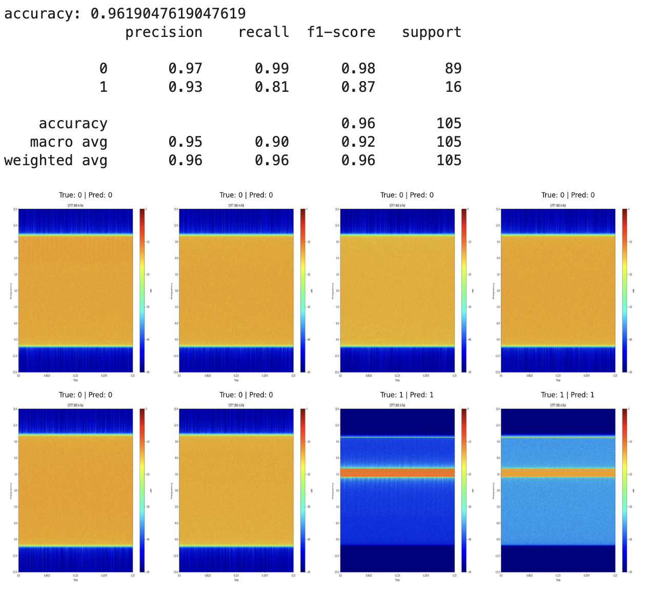
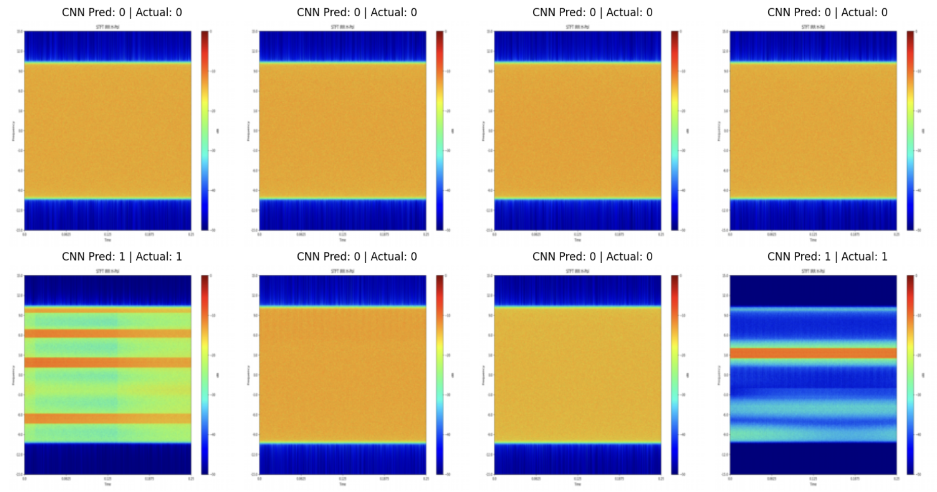
  1. Trained a CNN for RFI detection using pre-trained model (ResNet18) with the last classification layer modified
  2. Developed an SVM baseline to assess the efficiency of the CNN approach (address potential underutilization of the neural network)
     • Performed cross-validation to ensure the models were not overfitting
     • Both the CNN and SVM achieved over 95% accuracy, correctly labeling each graph as either 0 = clean or 1 = RFI

• Continued obtaining data from transition band (100 additional rows: 1413.5mHz(fc0), 1453.5mHz(fc4)
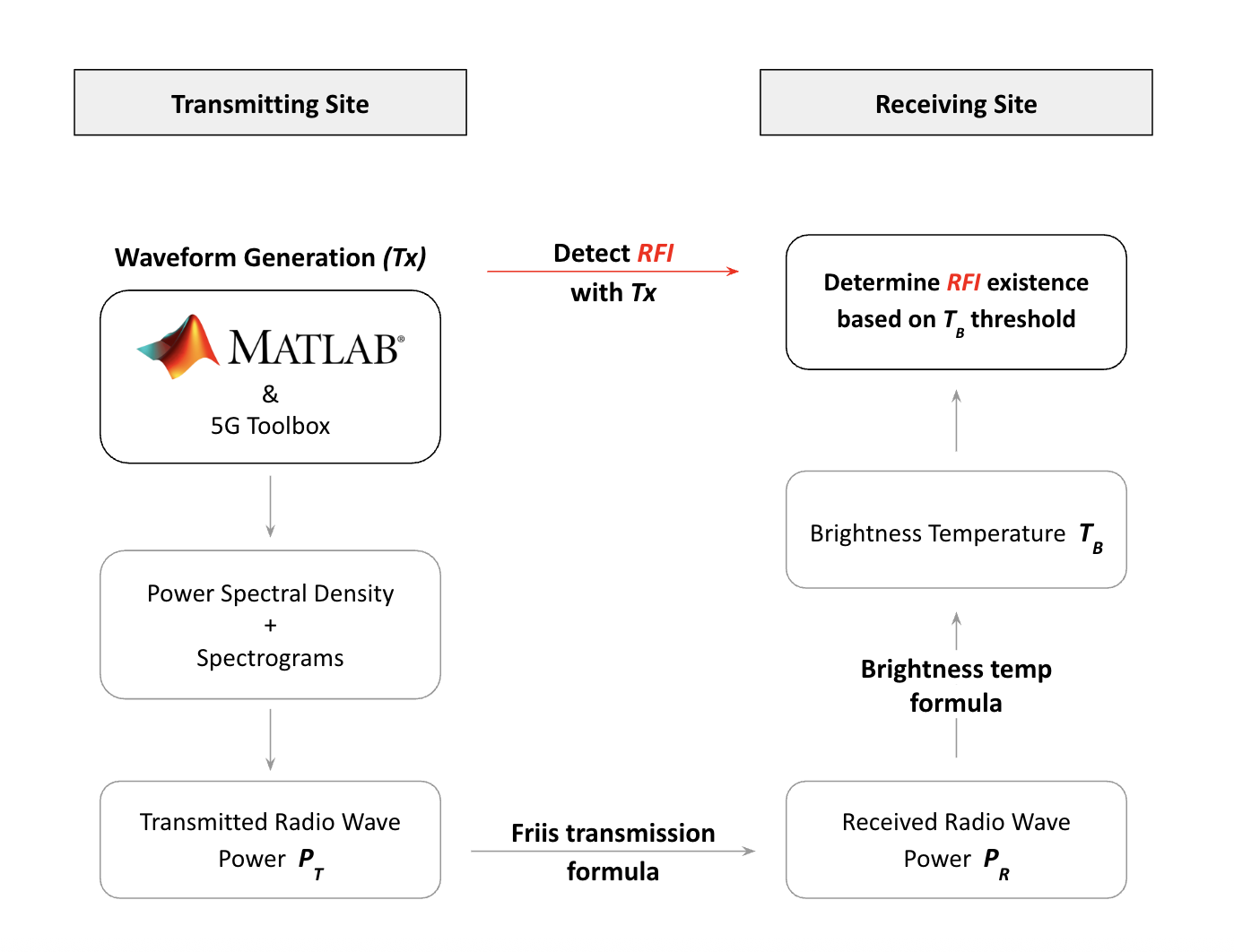
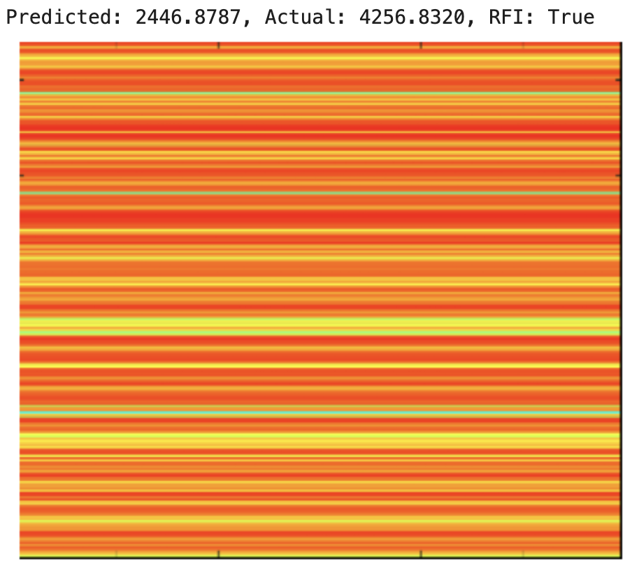
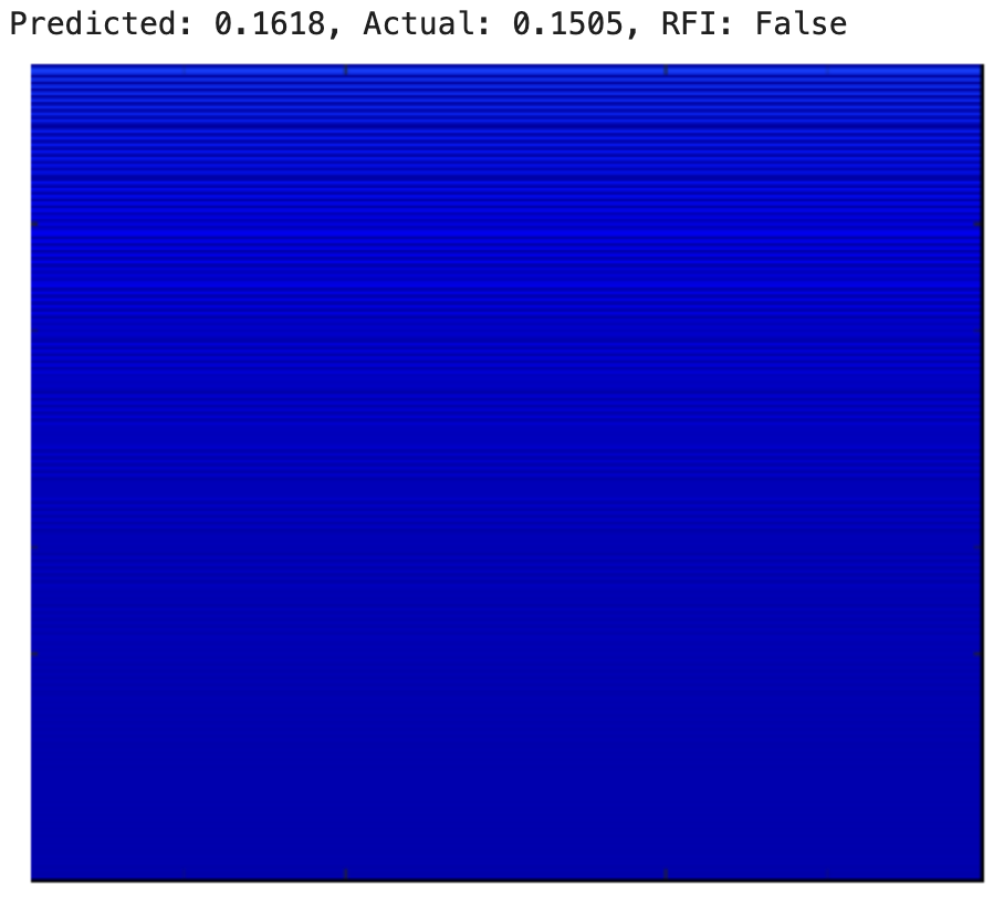
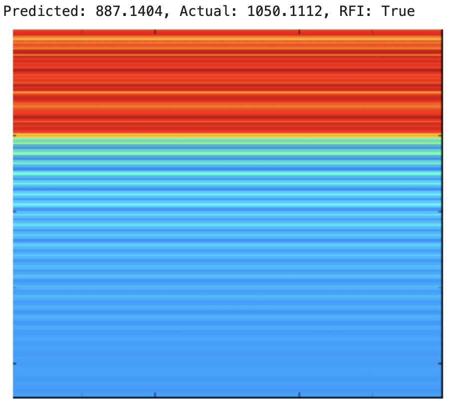
• Created a mathematical pipeline to estimate brightness temperature(K) based on total transmitting power(W)
  • Approximate amount of received power from total transmitted power using Friis Transmission formula
  • Use power recieved to estimate change in brightness temperature cause by RFI

Week 8 (7/14 - 7/17):